Analysis of QA vacuum equilibrium

import numpy as np
import matplotlib.pyplot as plt

from spectre import SPECTREout

%matplotlib inline

np.set_printoptions(linewidth=170)

# Load the output file(s) into custom object(s)

obj_opt = SPECTREout("init_opt.h5")
obj_init = SPECTREout("init.h5")

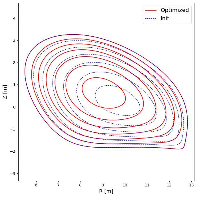
fig, ax = plt.subplots(figsize=(7, 7))

zetan = 0.4  # Zeta normalized to one field period

obj_opt.plot_infaces(color="r", ax=ax, zetan=zetan, label="Optimized")  # Plot interfaces
obj_opt.plot_poincare(ax=ax, zetan=zetan)  # Plot poincare tracing

obj_init.plot_infaces(color="b", lw=0.9, ls="--", ax=ax, zetan=zetan, label="Init")

ax.legend(fontsize=14)

plt.tight_layout()

plt.show()

obj_opt.plot_pressure()

plt.tight_layout()

plt.show()

# Get coordinates at any point
lvol = 1
sarr = np.linspace(-0.9, 0.8, 2)
tarr = np.linspace(0.1, 3.0, 3)
zarr = np.array([0.2])
rarr, zarr = obj_opt.get_coord_transform(
    lvol, sarr, tarr, zarr
)  # Get R, Z coordinates from s, theta, zeta coordinates
"R: ", rarr[0], "Z: ", zarr[0]

('R: ',
 array([[[12.96477979],
         [12.70767649],
         [12.22959498]],
 
        [[13.23615815],
         [12.45285811],
         [12.03054319]]]),
 'Z: ',
 array([[[ 0.30892629],
         [-1.32686525],
         [ 0.46901512]],
 
        [[ 0.01539442],
         [-2.60344226],
         [ 0.36263902]]]))

# Get field modulus at any point
lvol = 1
sarr = np.linspace(-0.9, 0.8, 2)
tarr = np.linspace(0.1, 3.0, 3)
zarr = np.array([0.2])
(
    obj_opt.get_field_mod(lvol, sarr, tarr, zarr),
    obj_opt.get_field_contrav(lvol, sarr, tarr, zarr)[0],
)  # Get the field at some s, theta, zeta

(array([[[4.68385741],
         [4.92803359],
         [5.1598008 ]],
 
        [[4.55117254],
         [4.99335211],
         [5.34200459]]]),
 array([[[ 0.00678082],
         [-0.0126568 ],
         [-0.00081595]],
 
        [[ 0.00900606],
         [-0.02314996],
         [-0.00177068]]]))